Physicist: The Monogamy of Entanglement is the statement that “maximally entangled” particles only show up in pairs. Entanglement is a sliding scale, so things can be non-entangled or a little entangled, but when the quantum states of two things are completely tied up in each other, there’s just no room for a third. This is more about how entanglement is defined mathematically and less about a dramatic insight into the true nature of reality.

Monogamy of Entanglement: Two maximally entangled particles cannot be entangled with any others. But the exact meaning of entanglement, like matrimony, is a matter of definition.
One particle: Quantum stuff can be (and generally is) in a “superposition”, multiple states at the same time. For example, an electron belonging to Alice (or anyone else), can be both “spin up” and “spin down” in equal parts; a superposition that’s written 


Now here’s the thing. Quantum randomness is relative. One person’s superposition is another person’s definite state. For example, that superposition from earlier is also a definite state 

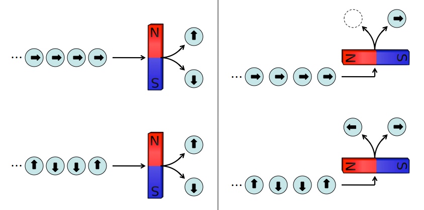
Spin causes particles to act like tiny magnets, which gives us a handy way to measure it. Left: When you measure spin vertically, there’s no way to tell the difference between a string of spin right electrons (top) and a string of random spin up/down electrons (bottom). Right: But if you measure horizontally, the string of spin right electrons always get sorted correctly, while the up/down electrons continue to produce random results.
If some devious ne’er-do-well sent you a never-ending stream of
Here’s the point. If you’re always looking at the same, definite state, then you should be able to find some measurement that always produces a definite result. But if you’re being fed a random set of states, there’s no way to do a measurement that produces consistent results. I suppose you could turn the detector off and walk away, but that’s dirty pool.
Quick aside: I’m dropping the coefficients in front of the states that would normally dictate their probability of being measured (the state 
Two Particles: When you need to worry about multiple systems (particles, quantum computers, needlessly diverse collections of scarves, or whatever else), you don’t worry about their individual superpositions of states, you worry about superpositions of their collective states. So if you have a second electron, under the custodianship of Bob, you wouldn’t first talk about the states of Alice’s electron (


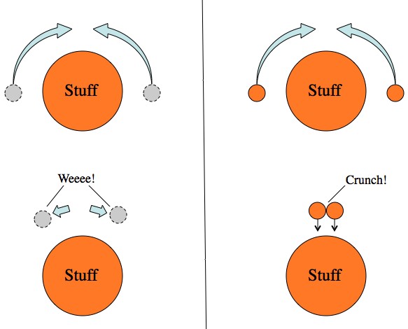
Left: In classical physics a system’s state is the aggregation of each part taken individually. Right: In quantum physics the system as a whole has a state that’s shared between each part.
For example, if both electrons are in the same equal superposition of spin up and down from earlier, then their collective state is
\left(|\uparrow\rangle_B+|\downarrow\rangle_B\right)=|\uparrow\rangle_A|\uparrow\rangle_B+|\downarrow\rangle_A|\uparrow\rangle_B+|\uparrow\rangle_A|\downarrow\rangle_B+|\downarrow\rangle_A|\downarrow\rangle_B")
If Alice measures her electron and finds that it’s spin up, then the state of the pair is now
")
and if she finds that her electron is spin down, then the overall state is
")
In other words, in this situation it doesn’t matter what Alice sees; Bob’s state is independent of it. This particular collective state can be described first by considering Alice’s electron and then considering Bob’s (or vice versa), because knowing the result of a measurement on one part tells you nothing about what you’ll see when you measure the other. A state like this is called “separable”, because it can be separated mathematically. Physicists are very clever namers of things, which is why they often refer to themselves as namerators.
Non-seperable states are entangled; a measurement on one part gives you information about what the result of a measurement on another part will be. For example,

is definitely not separable. If Alice were to measure her electron the state of the system as a whole would be either
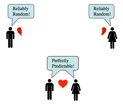
In other words, by looking at her own electron, Alice knows what Bob will measure, whenever he gets around to it. This state is “maximally entangled” because knowing one measurement allows you to perfectly predict the other.
But once Alice has measured her electron, and the system as a whole is now either 
This randomness isn’t a symptom of Alice having done a measurement, it’s a feature of entangled states in general. After all, Bob and his pet electron could be anywhere. Despite the nearly universal, but categorically false, belief that entangled particles affect each other, nothing that Alice does or doesn’t do with her electron will ever have any impact on Bob’s electron.
If Alice measures her particle, Bob gets a random result. But since the particles can’t communicate and it doesn’t actually matter what Alice does, Bob gets a random result anyway.
Entangled particles follow the same rule that single particles follow: wrong measurement = random result, correct measurement = definite result. But in order to do the “correct measurement” you always need to have access to the entire state. If you have both entangled particles in front of you, then you can easily do a measurement to determine which maximally entangled state you have (for example 
If you only have access to part of an entangled state, you’ll get random results no matter how you measure it. But if you have access to all of an entangled state, there is a “correct” measurement with predictable results.
This leads to a rather profound fact: entangled states always appear random when you only measure part of them. That is, they never seem to be in a superposition of states, they always appear to be a randomly selected state, since there’s no measurement that makes them predictable (see the one particle case).
There are still some clever things you can do with entangled particles that take advantage of their quantum correlations, like quantum teleportation, but two facts remain immutable: 1) when you measure one particle alone the result is random and 2) the two particles never ever influence each other in any way.
How entanglement is defined: When you don’t have access to both entangled particles and are forced to measure them one at a time, you get random results. You can describe how random those results are in terms of how much information it takes to describe them: two possible results (up or down) takes 1 bit of information (0 or 1). When you do have access to both entangled particles, you can do a measurement that will always produce the same, predictable result. One possible result takes zero bits of information. After all, if you had flipped a two-headed coin, would you really need to write down the results at all? Zero bits.
This difference between the randomness of the particles when they’re apart minus the randomness when they’re together is how entanglement is defined. A maximally entangled pair of particles has “1 ebit” of entanglement and a separable pair of particles has 0 ebits.
And yes, there are states in between. For example, 
Three Particles: If Alice’s electron is in a superposition of spin up and down, its state is
So what’s stopping Carol and her electron from also being both spin up and down in tandem with Alice and Bob’s? Not a damn thing.

Today we can create states like this with not just three, but dozens of particles. No big deal. Any reasonable person (with at least a passing familiarity with quantum notation) would say that state looks pretty entangled.
If Carol measures the spin of her electron, then the state of the system goes from 

With the third-act-introduction of Carol, suddenly they’re working with one of two randomly selected states (
However! Entanglement is narrowly defined is in terms of how much more random your particles are when they’re apart vs. when they are together. Same amount of randomness means zero entanglement. So because there’s a third (or fourth or fifth…) party involved the state, no two parts can be maximally entangled.
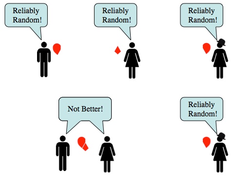
Entangled states are random apart and predictable together. That difference is how entanglement is defined. If a state is divided among more than two places, no pair can have the whole state, so the results are always random.
So it’s not that you can’t do fancy quantum states with many particles at once, and it’s not that something terribly profound happens when you move from using two particles to using three, but going by the stringent definition of entanglement: if two parties share a maximally entangled state with each other, they don’t share it with anyone else. One might even go so far as to say that entanglement is monogamous.
Like many seemingly arbitrary mathematical definitions, it turns out that the monogamy of entanglement is a powerful, useful statement. It is the key behind why quantum security is so secure (and quantum). By sharing a string of maximally entangled states with each other, then measuring some and sharing the results, Alice and Bob can check to see if there’s a third party corrupting their state. If there isn’t, they can dive into their private conversation. If there is, then they’ve caught themselves an eavesdropper. Quantum cryptography is Carol-proof!


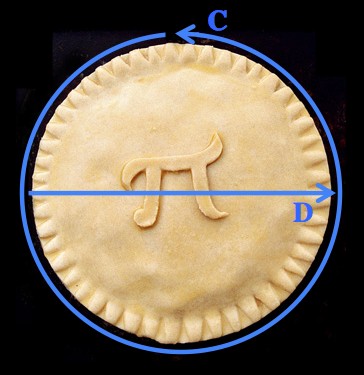
 , an approximation within half a percent of the correct value. Which, for the bronze age, is fine.
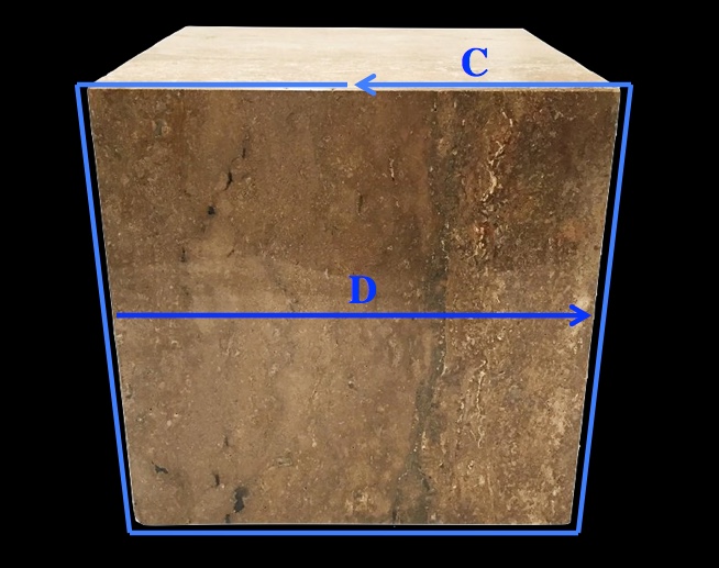
 . If you want to predict how much water a cylindrical barrel can hold to within a couple percent, then you need to know π to at least a couple digits.

(3)}{3.46+3}\approx3.215")
(3.215)}\approx3.106")
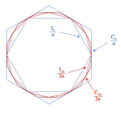
 for all n, this gives us an ever-diminishing range where π can be found. Here’s why it works:
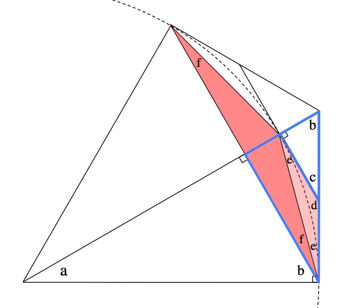
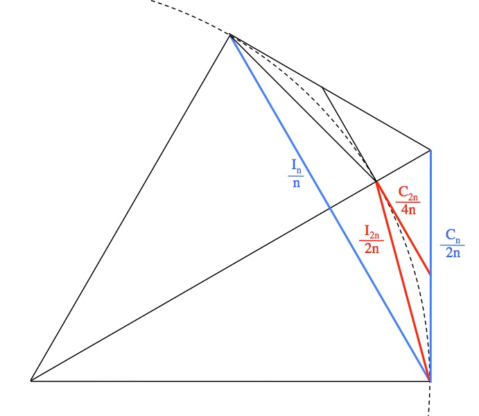
![\begin{array}{rcl} \frac{\left(\frac{C_n}{2n}\right)}{\left(\frac{I_n}{2n}\right)}&=&\frac{\left(\frac{C_n}{2n}-\frac{C_{2n}}{4n}\right)}{\left(\frac{C_{2n}}{4n}\right)} \\[4mm] \frac{C_n}{I_n}&=&\frac{2C_n-C_{2n}}{C_{2n}} \\[2mm] \frac{C_n}{I_n}&=&\frac{2C_n}{C_{2n}}-1 \\[2mm] \frac{C_n}{I_n}+1&=&\frac{2C_n}{C_{2n}} \\[2mm] C_n+I_n&=&\frac{2C_nI_n}{C_{2n}} \\[2mm] C_{2n}\left(C_n+I_n\right)&=&2C_nI_n \\[2mm] C_{2n}&=&\frac{2C_nI_n}{C_n+I_n} \\[2mm] \end{array}](https://s0.wp.com/latex.php?latex=%5Cbegin%7Barray%7D%7Brcl%7D+%5Cfrac%7B%5Cleft%28%5Cfrac%7BC_n%7D%7B2n%7D%5Cright%29%7D%7B%5Cleft%28%5Cfrac%7BI_n%7D%7B2n%7D%5Cright%29%7D%26%3D%26%5Cfrac%7B%5Cleft%28%5Cfrac%7BC_n%7D%7B2n%7D-%5Cfrac%7BC_%7B2n%7D%7D%7B4n%7D%5Cright%29%7D%7B%5Cleft%28%5Cfrac%7BC_%7B2n%7D%7D%7B4n%7D%5Cright%29%7D+%5C%5C%5B4mm%5D+%5Cfrac%7BC_n%7D%7BI_n%7D%26%3D%26%5Cfrac%7B2C_n-C_%7B2n%7D%7D%7BC_%7B2n%7D%7D+%5C%5C%5B2mm%5D+%5Cfrac%7BC_n%7D%7BI_n%7D%26%3D%26%5Cfrac%7B2C_n%7D%7BC_%7B2n%7D%7D-1+%5C%5C%5B2mm%5D+%5Cfrac%7BC_n%7D%7BI_n%7D%2B1%26%3D%26%5Cfrac%7B2C_n%7D%7BC_%7B2n%7D%7D+%5C%5C%5B2mm%5D+C_n%2BI_n%26%3D%26%5Cfrac%7B2C_nI_n%7D%7BC_%7B2n%7D%7D+%5C%5C%5B2mm%5D+C_%7B2n%7D%5Cleft%28C_n%2BI_n%5Cright%29%26%3D%262C_nI_n+%5C%5C%5B2mm%5D+C_%7B2n%7D%26%3D%26%5Cfrac%7B2C_nI_n%7D%7BC_n%2BI_n%7D+%5C%5C%5B2mm%5D+%5Cend%7Barray%7D&bg=ffffff&fg=000&s=0&c=20201002)
![\begin{array}{rcl} \frac{\left(\frac{I_{2n}}{2n}\right)}{\left(\frac{C_{2n}}{4n}\right)}&=&\frac{\left(\frac{I_n}{n}\right)}{\left(\frac{I_{2n}}{2n}\right)} \\[4mm] \frac{I_{2n}}{C_{2n}}&=&\frac{I_n}{I_{2n}} \\[2mm] \left(I_{2n}\right)^2&=&I_nC_{2n} \\[2mm] I_{2n}&=&\sqrt{I_nC_{2n}} \\[2mm] \end{array}](https://s0.wp.com/latex.php?latex=%5Cbegin%7Barray%7D%7Brcl%7D+%5Cfrac%7B%5Cleft%28%5Cfrac%7BI_%7B2n%7D%7D%7B2n%7D%5Cright%29%7D%7B%5Cleft%28%5Cfrac%7BC_%7B2n%7D%7D%7B4n%7D%5Cright%29%7D%26%3D%26%5Cfrac%7B%5Cleft%28%5Cfrac%7BI_n%7D%7Bn%7D%5Cright%29%7D%7B%5Cleft%28%5Cfrac%7BI_%7B2n%7D%7D%7B2n%7D%5Cright%29%7D+%5C%5C%5B4mm%5D+%5Cfrac%7BI_%7B2n%7D%7D%7BC_%7B2n%7D%7D%26%3D%26%5Cfrac%7BI_n%7D%7BI_%7B2n%7D%7D+%5C%5C%5B2mm%5D+%5Cleft%28I_%7B2n%7D%5Cright%29%5E2%26%3D%26I_nC_%7B2n%7D+%5C%5C%5B2mm%5D+I_%7B2n%7D%26%3D%26%5Csqrt%7BI_nC_%7B2n%7D%7D+%5C%5C%5B2mm%5D+%5Cend%7Barray%7D&bg=ffffff&fg=000&s=0&c=20201002)
") and what you get will be a number closer to
and what you get will be a number closer to  than your original guess, x. This method was known to the Babylonians and Archimedes (it is, in fact, “the Babylonian method”) and it converges quadratically, so it achieves whatever (reasonable) accuracy you’re hoping for almost instantly.
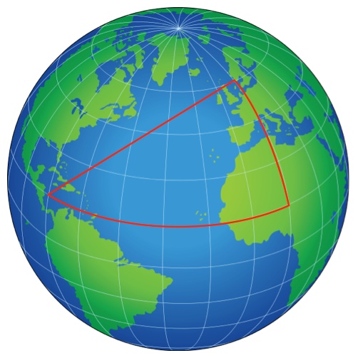
") .
.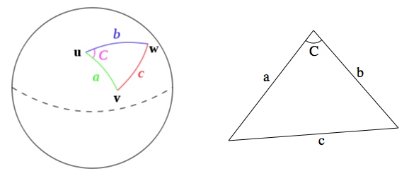
=\cos(a)\cos(b)+\sin(a)\sin(b)\cos(C)")
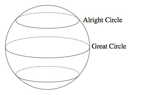
 . This is generally easier to use than the actual distance. For example, the angle from the north pole to the equator is 90° (obviously) while the physical distance is about 6,200 miles (different on every planet).
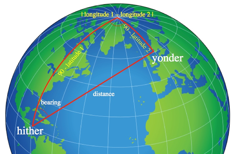
 :
: ") ,
, ") , and
, and  .
.=\cos\left(\theta_1\right)\cos(\theta_2)+\sin\left(\theta_1\right)\sin(\theta_2)\cos(\phi)")
![\textrm{distance}=(\textrm{Earth's radius})\arccos\left[\cos\left(\theta_1\right)\cos(\theta_2)+\sin\left(\theta_1\right)\sin(\theta_2)\cos(\phi)\right]](https://s0.wp.com/latex.php?latex=%5Ctextrm%7Bdistance%7D%3D%28%5Ctextrm%7BEarth%27s+radius%7D%29%5Carccos%5Cleft%5B%5Ccos%5Cleft%28%5Ctheta_1%5Cright%29%5Ccos%28%5Ctheta_2%29%2B%5Csin%5Cleft%28%5Ctheta_1%5Cright%29%5Csin%28%5Ctheta_2%29%5Ccos%28%5Cphi%29%5Cright%5D&bg=ffffff&fg=000000&s=0 "\textrm{distance}=(\textrm{Earth's radius})\arccos\left[\cos\left(\theta_1\right)\cos(\theta_2)+\sin\left(\theta_1\right)\sin(\theta_2)\cos(\phi)\right]")
=\cos\left(\theta_1\right)\cos\left(\frac{\textrm{distance}}{\textrm{Earth's radius}}\right)+\sin\left(\theta_1\right)\sin\left(\frac{\textrm{distance}}{\textrm{Earth's radius}}\right)\cos\left(\textrm{bearing}\right)")
![\textrm{bearing}=\arccos\left[\frac{\cos\left(\theta_2\right)-\cos\left(\theta_1\right)\cos\left(\frac{\textrm{distance}}{\textrm{Earth's radius}}\right)}{\sin\left(\theta_1\right)\sin\left(\frac{\textrm{distance}}{\textrm{Earth's radius}}\right)}\right]](https://s0.wp.com/latex.php?latex=%5Ctextrm%7Bbearing%7D%3D%5Carccos%5Cleft%5B%5Cfrac%7B%5Ccos%5Cleft%28%5Ctheta_2%5Cright%29-%5Ccos%5Cleft%28%5Ctheta_1%5Cright%29%5Ccos%5Cleft%28%5Cfrac%7B%5Ctextrm%7Bdistance%7D%7D%7B%5Ctextrm%7BEarth%27s+radius%7D%7D%5Cright%29%7D%7B%5Csin%5Cleft%28%5Ctheta_1%5Cright%29%5Csin%5Cleft%28%5Cfrac%7B%5Ctextrm%7Bdistance%7D%7D%7B%5Ctextrm%7BEarth%27s+radius%7D%7D%5Cright%29%7D%5Cright%5D&bg=ffffff&fg=000000&s=0 "\textrm{bearing}=\arccos\left[\frac{\cos\left(\theta_2\right)-\cos\left(\theta_1\right)\cos\left(\frac{\textrm{distance}}{\textrm{Earth's radius}}\right)}{\sin\left(\theta_1\right)\sin\left(\frac{\textrm{distance}}{\textrm{Earth's radius}}\right)}\right]")
\approx1.367") ,
, \approx0.530") , and
, and \right|\approx1.593") . So the distance is
. So the distance is![\textrm{distance}=(3959miles)\arccos\left[\cos\left(1.367\right)\cos(0.530)+\sin\left(1.367\right)\sin(0.530)\cos(1.593)\right]=(3959miles)(1.406)=5566miles](https://s0.wp.com/latex.php?latex=%5Ctextrm%7Bdistance%7D%3D%283959miles%29%5Carccos%5Cleft%5B%5Ccos%5Cleft%281.367%5Cright%29%5Ccos%280.530%29%2B%5Csin%5Cleft%281.367%5Cright%29%5Csin%280.530%29%5Ccos%281.593%29%5Cright%5D%3D%283959miles%29%281.406%29%3D5566miles&bg=ffffff&fg=000000&s=0 "\textrm{distance}=(3959miles)\arccos\left[\cos\left(1.367\right)\cos(0.530)+\sin\left(1.367\right)\sin(0.530)\cos(1.593)\right]=(3959miles)(1.406)=5566miles")
![\textrm{bearing}=\arccos\left[\frac{\cos\left(0.530\right)-\cos\left(1.367\right)\cos\left(\frac{5566}{3959}\right)}{\sin\left(1.367\right)\sin\left(\frac{5566}{3959}\right)}\right]=0.538rad=30.1^o](https://s0.wp.com/latex.php?latex=%5Ctextrm%7Bbearing%7D%3D%5Carccos%5Cleft%5B%5Cfrac%7B%5Ccos%5Cleft%280.530%5Cright%29-%5Ccos%5Cleft%281.367%5Cright%29%5Ccos%5Cleft%28%5Cfrac%7B5566%7D%7B3959%7D%5Cright%29%7D%7B%5Csin%5Cleft%281.367%5Cright%29%5Csin%5Cleft%28%5Cfrac%7B5566%7D%7B3959%7D%5Cright%29%7D%5Cright%5D%3D0.538rad%3D30.1%5Eo&bg=ffffff&fg=000000&s=0 "\textrm{bearing}=\arccos\left[\frac{\cos\left(0.530\right)-\cos\left(1.367\right)\cos\left(\frac{5566}{3959}\right)}{\sin\left(1.367\right)\sin\left(\frac{5566}{3959}\right)}\right]=0.538rad=30.1^o")
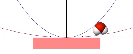
 (There’s nothing too special about parabolas; every curve that doesn’t have sharp corners can be closely approximated by circles and vice versa, it’s just that parabola math is easy). Spoons have a radius of around 1 cm. Bowls have a radius of around 7 cm. The distance from the center (the point of contact) to the edge of the strip, x, such that water molecules won’t be able to slip through the gap between the bowl and the passing spoon is given by
 }x^2-\frac{1}{2(0.07m)}x^2=0.25\times10^{-9}m") . Solve for x and you get
. Solve for x and you get  , so the strip should be about 5 micrometers across; on the order of a tenth of a hair’s width.