Physicist: What follows is the famous Shor algorithm, which can break any RSA encryption key.
The problem: RSA, the most common form of public key encryption, is based on the fact that large numbers are hard to factor. Without going into too much detail, an encryption key M, is the product of two large primes P and Q (M=PQ), and breaking the key comes down to finding P and Q, given M. This is difficult and can’t be done in any reasonable time for large values of M.
For example, M=6563955109193980058697529924699940996676491413219355771. What are P and Q?
(ans: 8764325985409367513190343 and 748940091927375783904810247597. Prime numbers supplied by numberempire.com)
One method involves modular arithmetic. In modular math you take a number, M, and every time you deal with a number larger than M, you subtract M until you’re dealing with a number smaller than M. Clocks are the most commonly seen example of “mod 12” arithmetic. For example, 31 o’clock is the same as 19 o’clock is the same as 7 o’clock.
You could re-write that as . There’s a lot of interesting stuff (card tricks) involving modular math in this older post, so if you’re not familiar with modular math jump over there real quick.
Now check this out:
This pattern: 1,2,4,8,1,2,4,8,1,… will repeat forever. Here’s why that’s useful. For a given A (it doesn’t really matter what A is), if you can find the lowest value, r, for which then, if r is even, you can do this:
If r isn’t even you change A and try again. When you say something is equal to , what you mean is that it’s a multiple of M. So
and
have factors in common with M, and yet (for mathy reasons) neither of them is a multiple of M on its own.
So in the “15” example, A=2, M=15, and r=4.
Boom! There are your factors! P=3 and Q=5.
For large values of M however, you can’t just raise A to higher and higher powers and wait until . Heavens no. For example, if you were trying this technique on the M from the top of this section you’d find that
.
It’s easy to raise A to a large power once, but there isn’t enough time in the universe to raise it to every power up to some huge number.
Enter quantum computing. A quantum computer has no problem raising A to many, many powers at the same time.
The solution (The Shor algorithm): So the name of the game is to find that “r” value. It has two properties: it’s the smallest number such that , and as you raise A to higher and higher powers r is how long it takes for the pattern to repeat (like in the “15” example; 1,2,4,8,1,2,4,8,…).
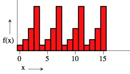
2^x mod 15. This is the example used to demonstrate the Shor algorithm below. The important thing to notice is that the function repeats.
In a nutshell: You’d like to find the value of r such that the function () repeats every r, so that you can do the “
” trick. Since this function has such a nice, repeating pattern the “Fourier transform” is very sharp. The Fourier transform breaks down signals into their component frequencies, and a repeating function has a very definite frequency. You can use that frequency to give you r. The smaller r is, the faster the function repeats, and the higher the frequency, and the larger r is, the slower the function repeats, and the lower the frequency.
So why do you need a quantum computer to do this? You need the function to exist in the computer all at once. If (like in a conventional computer) you can only have one value at a time, suddenly it doesn’t make sense to talk about the “frequency” of the function.
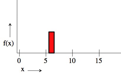
A classical computer can only see one value of x at a time, so there's no sense talking about "repeating" and "frequencies". A normal computer can do many values in a row, and different computers can handle different values at the same time, but you need a quantum computer to have multiple values in the same processor.
In what follows I’ll go through the algorithm step by step, then run through an example (factoring 15), indicated by italics. It’s not necessary to understand all of the math in detail to understand the ideas. So please: don’t stress.
The computer starts with two registers. In what follows the notation “” means the first register holds a 1 and the second register holds a 2. Several of these added together means that the computer is in multiple states at the same time. For example: “
” means that the computer is holding two states at the same time. 1 and 3 in the first register, 2 and 4 in the second register.
Step 1) Initialize the first register to an equal super-position of every possible number from 0 to N, where N is some power of 2 that’s larger than M2, and initialize the second register to zero.
N has to be a power of 2 because it’s dictated by the number of qbits in the first register, but for now, the only thing that’s important is that N is big.
The quantum state looks like this: .
In practice, for M=15, you’d want N>225. But never mind that now, to save space we’ll use N=16. The initialized state looks like:
The “1/4” in front of each term is there because the probability of an event is the square of the probability amplitude, which is what we’re looking at. The “1/4” means that each term has a 1/16 ( = (1/4)2 ) chance of being measured, if you measured right now. Which you don’t.
Step 2) Define . Take the first register, run it through f, and put the result in the second register.
Now:
It doesn’t really matter what A you pick, so generally smaller, easier A’s are the way to go.
In this example, , so now you have:
The same repeating 1,2,4,8,… pattern shows up.
Step 3) “Look” at the second register. One of the incredibly awesome things about quantum computing is that it’s sometimes necessary to entangle the outside of the computer with part of the internal mechanism. You can describe this as “wave function collapse” or “projection” or whatever. In this case, it has the effect that the vast majority of states “vanish”, and that those that remain are spaced at a regular interval (which turns out to be the “r” that the algorithm is looking for). One of the clever things about the Shor algorithm is that it doesn’t matter what you see, just that it is seen. (It doesn’t have to be seen by a person or anything). Lets say that the observed value of f(x) is “B”. The new state looks like:
This is just the collection of all of the inputs that could have lead to f(x)=B, starting at the lowest value of x that could do it () and then every rth number after that.
Let’s say, for example, that you look at the second register and you see “8”. As a result the second register is in a “definite state” (), but the first register is still in a super-position of several states.
The states that “disappeared” are still being used. They’re just being used by different versions of you that saw different results (1, 2, and 4). That should be pretty off-putting, so just roll with it. Not that it matters, but in this case B=8, = 3, and r=4. This r is what the algorithm is looking for.
Step 4) Take the “quantum Fourier transform” of the first register. The Fourier transform takes in waves and spits out the frequencies of those waves. If you have a function, , then its Fourier transform is written “
” (read “f hat”). A good way to picture the Fourier transform is as a piano keyboard. Sound itself is just air moving back and forth (
), but if it’s moving back and forth quickly, then you must be playing the high keys (
).
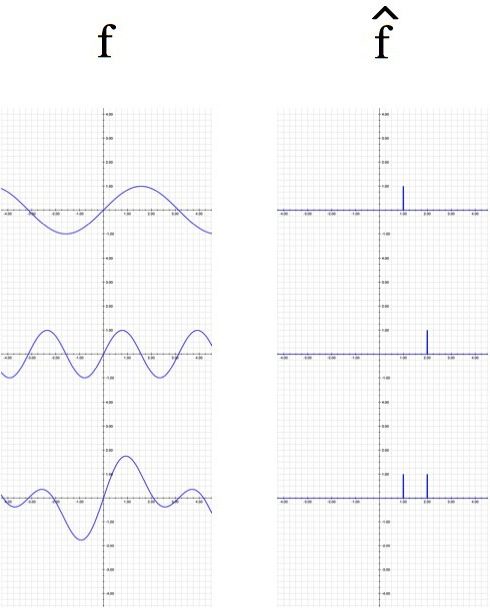
Functions (left column) and their Fourier transforms (right column): Sin(x), Sin(2x), and Sin(x)+Sin(2x)
In this case the pattern of numbers that exist in the first register are all evenly spaced (r apart). This is a very regular tone, so the Fourier transform will have sharp spikes like the examples in the picture above. The new state, after the quantum Fourier transform is:
The Fourier transform is the part of this process that takes advantage of constructive and destructive interference.
The Fourier transform of the example state in step 3 is:
Yes, those are imaginary i’s (as in ), but it’s cool. The probability is equal to the square of the absolute value of each of those numbers, and the absolute value of i is 1. So, for example,
. Each of these four values of k (0, 4, 8, and 12) has an equal one-in-four chance of being measured.
Step 5) Measure the first register. This will give you another number. The “spikiness” of the Fourier transform in the last step means that when you measure the value of the first register, you’ll be most likely to measure values of k such that is very near, or is equal to an integer. The last equation in step 4 is mostly fluff. The important part is the “
” part. When
is close to an integer, then this summation looks like “1+1+1+1+1….” and ends up very large. Otherwise, it ends up canceling itself out. For example, if
, then the summation becomes “1-1+1-1+1-1…”.
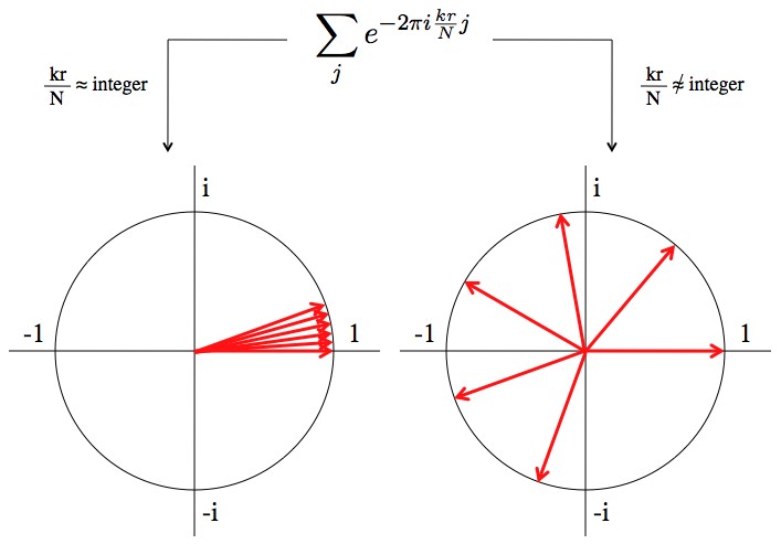
The important summation as seen in the complex plane. When kr/N is close to an integer every term in the summation "agrees" and makes the sum bigger. When kr/N is not close to an integer the terms of the sum "disagree" and the terms cancel each other out, leading to a very small total sum.
This is just the very mathematical side of saying “the Fourier transform is very spiked”. For a better understanding of this math, look up “complex plane“, “complex exponential“, and “geometric sum“.
The probability of measuring any of the values of the state is 1/4. Notice that each value of k makes
an integer! (remember that r=4 and N=16) Let’s say that (by random chance) we measure the first register and get k=12. It actually doesn’t matter which of the values we get (0, 4, 8, or 12), which is a big part of what makes this algorithm awesome (really awesome).
Step 6) Do some math. So, in step 5 you measure a value of k such that , where
is an integer. You know what N is (it’s the number of input states from step 1), and you know what k is (just measured it), but r and
are unknown. So what you’ve got is:
, an approximation of one rational number with another.
I didn’t want to make a big deal about it, but for the number, M, that you’re factoring, you’ll need N>M2. And, since M>r, N>r2 as well. It turns out that, given this condition, for a given value of k you’ll have a uniquely determined and r. You don’t care what
is, so chuck it out and keep r. The way you figure out what
is from
is by using a trick called “Approximation by Continued Fractions“.
In the last step the measured value was k=12. So, . In this case the approximation was exact, and r=4 and
=3 (not that it matters).
So, finally, r=4! We now know that . So:
We can now say, with heads held high, that 15 = 3×5. Tell your friends!
The “15” example is a little ideal (but also simple enough that you can look at each step in detail), so here’s one more example of the math with bigger numbers.
Say M=77, and you want to find the factors. Then you choose A=2 (because it’s easiest), and since M2=5929, you choose N = 8192 (a 13 bit register). You run through the algorithm and find that k=5188 (it could have been any one of many values, but this is what you got this time). Now you know that , where r<M. Using approximation by continued fractions you find that the closest values of
and r that work are
. So, your guess for r is r=30.
The two numbers you get are: [230/2-1]77 = [32767]77 = 42 and [230/2+1]77 = [32769]77 = 44. Now obviously, neither 42 nor 44 are factors of 77. However, they each share a factor in common with 77. All you have to do now is find the greatest common divisor (which is an extremely fast operation).
gcd(77,42) = 7
gcd(77,44) = 11
The Shor algorithm works perfectly (gives you a useful value of k) more than 40% of the time. That may not sound great. But if it doesn’t work the first time, why not try it a few thousand more times? On a quantum computer, this algorithm is effectively instantaneous.
I left a couple of details out of the math here because, frankly, this post is a little over the top. If you read all the way to here, buy yourself a drink and take a nap. However, if you’re interested in exactly why you need N>M2, how to execute the quantum Fourier transform, and why the algorithm works better than 40% of the time, then there are some rough notes in this pdf: Shor.
A commenter pointed out that the equations in this post may not be showing up for everyone. In partial remedy, here’s a pdf of the above post: quantum_RSA_Shor.





Pingback: Entanglement omnibus! | Ask a Mathematician / Ask a Physicist
Pingback: Q: How do you write algorithms to enycrypt things? | Ask a Mathematician / Ask a Physicist
Pingback: Q: Since the real-world does all kinds of crazy calculations in no time, can we use physics to calculate stuff? | Ask a Mathematician / Ask a Physicist
Pingback: Q: What is a Fourier transform? What is it used for? | Ask a Mathematician / Ask a Physicist
Pingback: The internet | When in doubt, bacon
Pingback: Episode 13: Quantum Computing | The Wonder of Reality
Pingback: Q: What is quantum supremacy? Is it awesome or worrisome? | Ask a Mathematician / Ask a Physicist